PROJECT 01
Quadruped Robotics
for Agricultural Sensing
Three connected research directions, from environmental mapping to crop observation. Select a card to explore each study.
Select a research area above to view its methods, figures and findings.
1. Greenhouse mapping
Greenhouse microclimate mapping using a quadruped robot to assess fixed sensor representativeness
Status: Manuscript in final preparation before submission.
Conference presentation: Park, S. (2026). Height-resolved 3D microclimate mapping and spatiotemporal analysis within greenhouse crop canopies using a quadruped robot. AKABFE Student Research Spotlight, ASABE Annual International Meeting, Indianapolis, USA.
This study examines how well fixed greenhouse sensors represent the microclimate across crop rows and canopy heights. A quadruped robot measured temperature, relative humidity and CO₂ to map spatial variation and compare mobile observations with fixed-sensor references.
Materials & Methods
The experiment took place in a cherry tomato glasshouse in Miryang, Republic of Korea. The robot surveyed eight 54 m pipe-rail lanes: L1–L4 beside dense canopies and L5–L8 beside pruned canopies. The two canopy conditions provided contrasting environments for interpreting the mapped measurements.
A Unitree Go2 EDU carried identical environmental sensing modules at the fruit zone (1.15 m) and upper canopy (1.65 m). Each module combined a BME280 temperature/humidity sensor and a CozIR-LP2 CO₂ sensor. An I²C multiplexer, Arduino Pro Mini and USB-to-TTL interface connected the two modules to the acquisition computer. Environmental readings were recorded at 2 Hz per height.
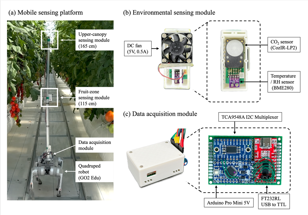
LiDAR-based rail detection and PID steering guided the forward measurement runs at 0.5 m/s. ROS 2 recorded the environmental and robot data against a common clock. Four sessions—morning, midday, afternoon and evening—were conducted once each on separate days between 9 and 12 June 2026.
Sensor cross-calibration aligned the two modules, and fixed-sensor time series were used to correct temporal variation during sequential lane surveys. Observations were averaged into 160 measured cells per map (eight lanes × 20 along-lane intervals), yielding 24 maps across three variables, two heights and four sessions. Along-lane coordinates were estimated from elapsed traversal time and lane length; no spatial interpolation was used to fill the maps.
Results
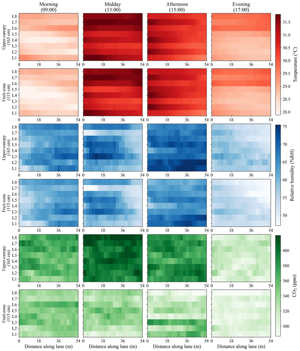
Spatial variation was consistently structured. All 24 maps showed positive spatial autocorrelation (Moran’s I 0.40–0.85; p < 0.001). Upper-canopy relative humidity exceeded fruit-zone values by 2.6–4.4 percentage points, and CO₂ was 12–69 ppm higher, in every session. At the upper canopy, the pruned section was warmer and drier than the dense section; canopy condition and location were confounded, so the difference cannot be attributed to pruning alone.
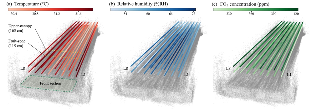
The spatial overlay connects environmental readings with crop-row geometry. Figure 6 locates the two-height measurements within the greenhouse structure and makes differences between lanes and canopy levels easier to interpret. Measurement positions are relative lane coordinates reconstructed from traversal time, rather than independently validated absolute positions.
Fixed readings did not fully represent the mobile spatial distributions. Humidity references were 2.4–7.3 percentage points below mobile means; CO₂ references were 48–116 ppm lower except in the evening. Depending on the session, 19–53% of cells differed from the fixed temperature reference by more than 0.5 °C, and 18–76% differed from the humidity reference by more than 5 percentage points.
The results support periodic mobile surveys to assess fixed-sensor representativeness and identify locations needing closer monitoring. They do not establish absolute sensor accuracy, energy savings or yield effects. Because the four sessions occurred on different days, session differences reflect both time of day and day-specific conditions.
My contribution
As a co-first author, I contributed to the methodology, experimental investigation and manuscript preparation.
2. Reservoirs
Quadruped-based Close-Range Upstream Surveys
Status: Completed.
Commissioning institution: National Disaster Management Research Institute (NDMI), Republic of Korea.
Contract research: Quadruped-based close-range soil surveys upstream of reservoirs, conducted under the project on integrated technology development for reservoir embankment risk prediction and maintenance management (Phase I).
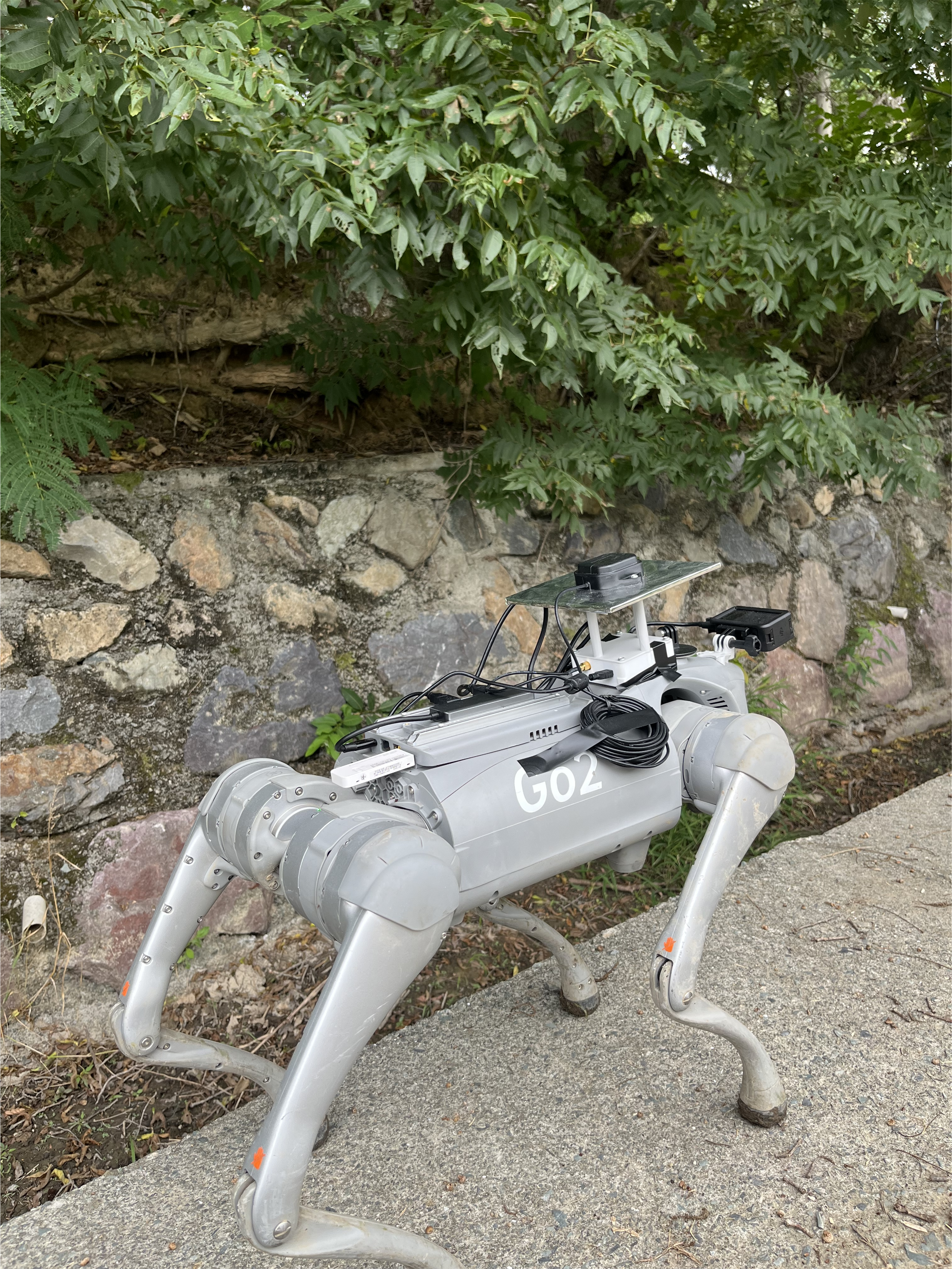
A quadruped robot was used to collect close-range images of exposed soil in the upstream areas of agricultural reservoirs before and after rainfall. The aim is to document ground-surface changes associated with soil erosion and sediment deposition. To support comparisons at corresponding locations across survey dates, the platform combined RTK-GNSS positioning with continuous RGB imaging from an action camera.
The recording system logged frame timestamps alongside GNSS observations in ROS 2. During post-processing, GNSS coordinates were interpolated to the frame timestamps, and selected frames were extracted with location metadata and displayed along the recorded survey routes. This provides a location-linked image dataset for repeated observation and subsequent analysis of rainfall-related surface changes.
Survey areas: upstream inflow areas of Hwangsaegol Reservoir (Miryang) and Dwitgol Reservoir (Ulsan).
| Condition | Hwangsaegol | Dwitgol |
|---|---|---|
| Dry | 2 Jul | 21 Jul |
| 30 Jul | 27 Jul | |
| — | 12 Aug | |
| Wet | 24 Aug | 24 Aug |
| 18 Sep | 18 Sep |
Camera height: 40 cm · Image scale: 0.23 mm/pixel
Field deployment
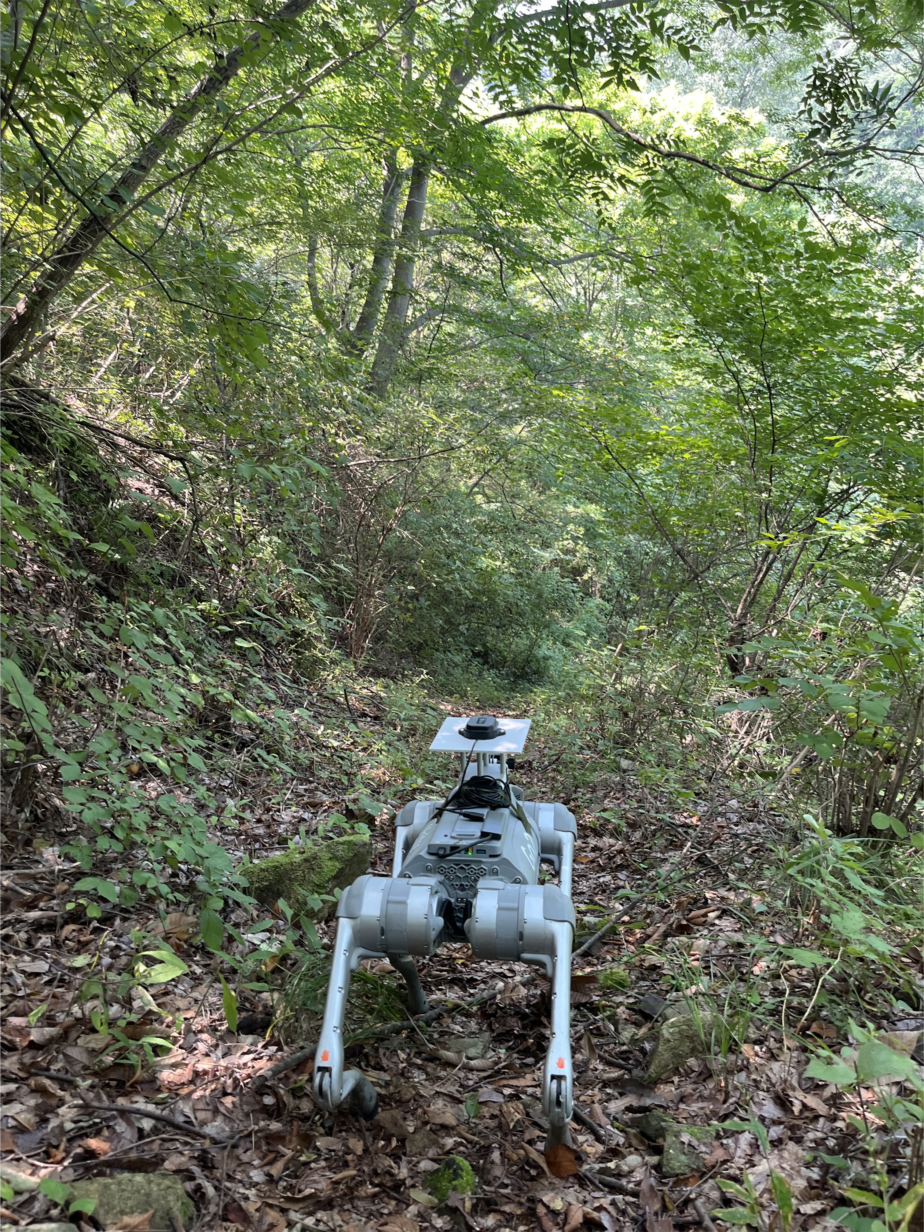
Survey sites and representative ground images
The coloured lines on each map show the quadruped robot’s recorded travel routes. Labels A–C mark the locations of the representative ground images.
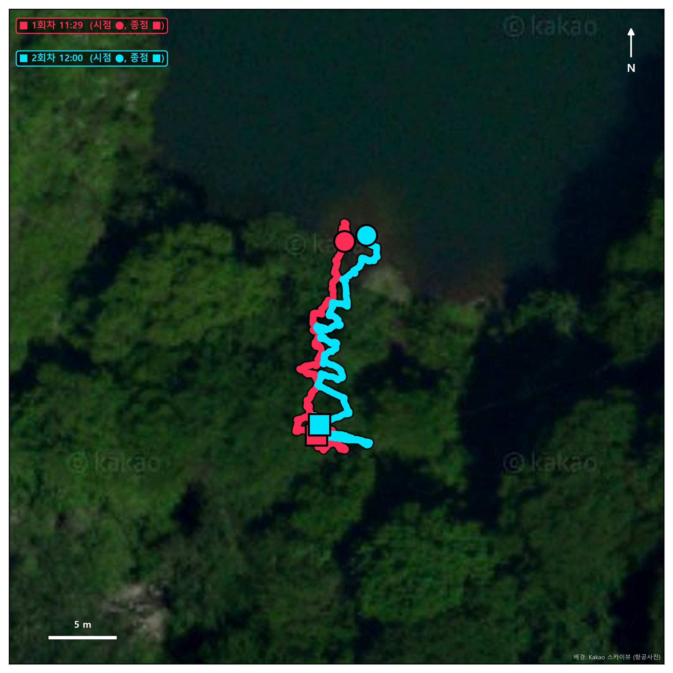
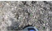
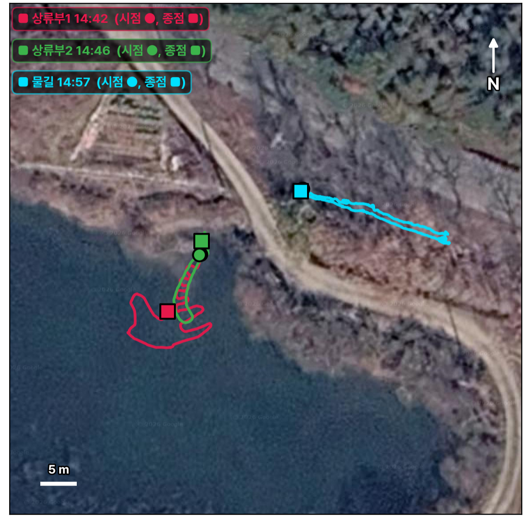
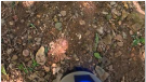
Image dataset
Extracted RGB frames are indexed by timestamp, latitude, longitude and cumulative travel distance, with image manifests and route maps for reviewing sample locations. A–C identify representative ground images. These outputs support spatially corresponding comparisons across surveys; precise repeat-location alignment and quantitative sediment-change assessment remain to be validated.
Image processing
Original RGB image → Surface classification → Isolated soil image


3. Plant phenotyping (M.S. Thesis Research)
Multi-scale soybean phenotyping with a quadruped robot and UAV
Status: Ongoing M.S. thesis research · Updated 14 October 2026.
My M.S. thesis investigates how field-scale UAV imagery and close-range quadruped RGB-D observations can describe complementary soybean traits before harvest. A drone maps the upper canopy across the field, while the robot observes plant bases and pods below the canopy. The study links these observations in common 1 m row segments and tests the robot estimates against manual measurements.
Field platform and data collection
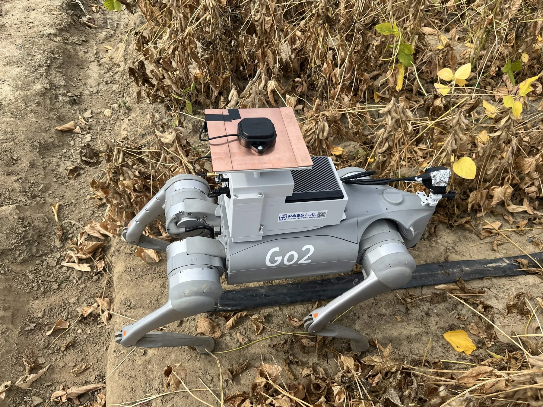
Ground platform: Unitree Go2 · RealSense D405 · MTi IMU · ZED-F9P RTK-GNSS · Jetson AGX Orin.
Aerial platform: DJI Mavic 3M with RGB and multispectral cameras. The soybean field is at the National Institute of Crop Science in Miryang, Republic of Korea.
UAV mapping with Agisoft Metashape
UAV imagery from 2 and 12 October 2026 was processed in Agisoft Metashape to reconstruct the field surface and produce RGB orthomosaics and digital surface models (DSMs). The outputs were resampled to a common local grid and oriented along the crop ridges for comparison with the robot surveys.
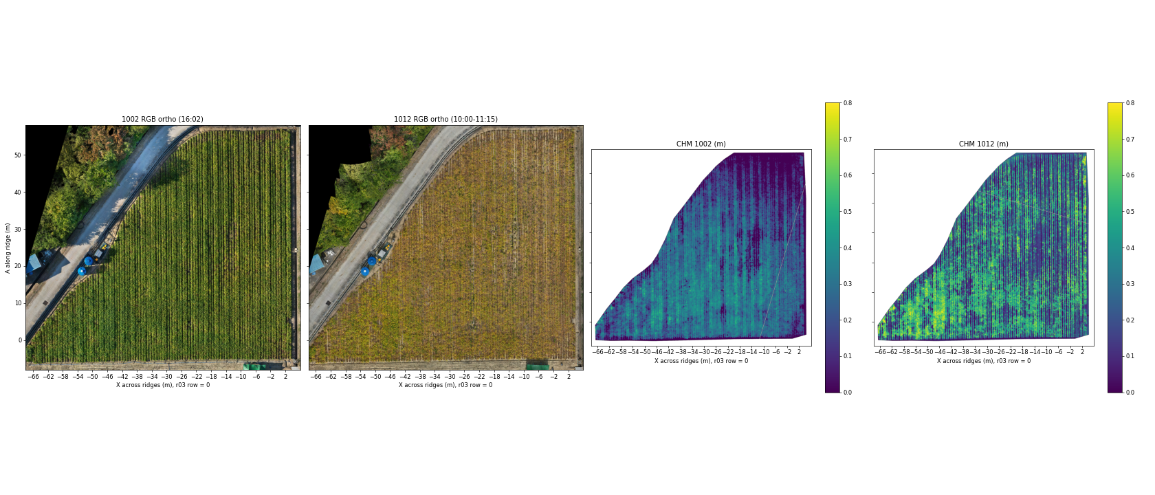
How the CHM was calculated. Canopy height is the DSM surface elevation minus the estimated local ground elevation. The initial Metashape ground classification included canopy in closed areas, so the ground model was rebuilt from low points in the 12 October DSM: the lowest 2% within 2 m × 2.8 m blocks, followed by removal of elevated blocks, interpolation and smoothing. These heights still require field validation and can reflect both plant height and leaf loss.
Selecting contrasting zones for robot surveys
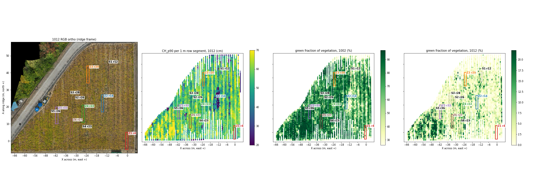
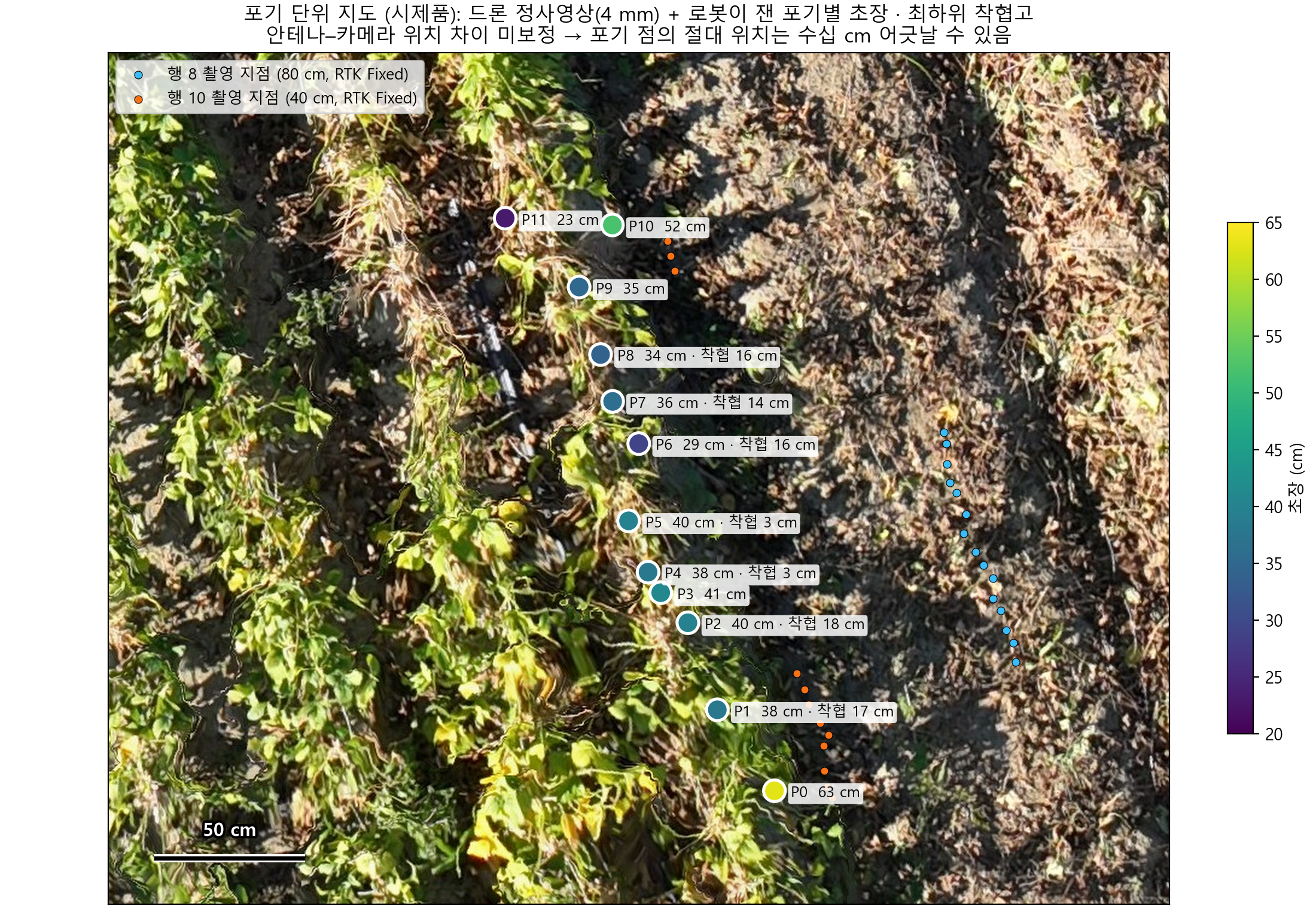
These maps guide the next ground campaign. Six 10 m candidate zones, including the previously surveyed r03 area, have been identified across the field's canopy-height and maturity gradient. Selection uses the 12 October 90th-percentile canopy height (CH_p90) and the 2 October RGB green fraction, choosing non-overlapping zones with relatively uniform conditions while covering the range from early leaf loss to retained green canopy. The 2 October CHM is excluded because its surface is smoothed and its vertical offset is inconsistent.
Zone selection and planned cross-scale validation
The current selection summarises 1 m × 0.70 m row segments, then compares 10 m windows using canopy height and RGB green fraction. A principal-component axis combines the two correlated indicators so that zones span their joint variation. Border ridges and the first and last 3 m of each ridge are excluded.
RTK-surveyed endpoints and ArUco markers at approximately 1 m intervals will connect UAV segments, robot imagery and sampled plants. The robot will survey the two rows from inside each ridge. Manual observations after the robot passes will record lowest pod-tip height, highest pod attachment height and plant height at marked sample plants. This will test measurement accuracy, repeatability and the effect of viewing only one side of each row.
Next UAV outputs: multispectral reflectance processing, NDVI/NDRE, vegetation cover and browning metrics will extend the segment table. NDVI and NDRE are planned outputs; they are not shown in the current RGB/CHM figures.
Connecting field maps to individual plants
Latest robot analysis: plant tracking and pod height
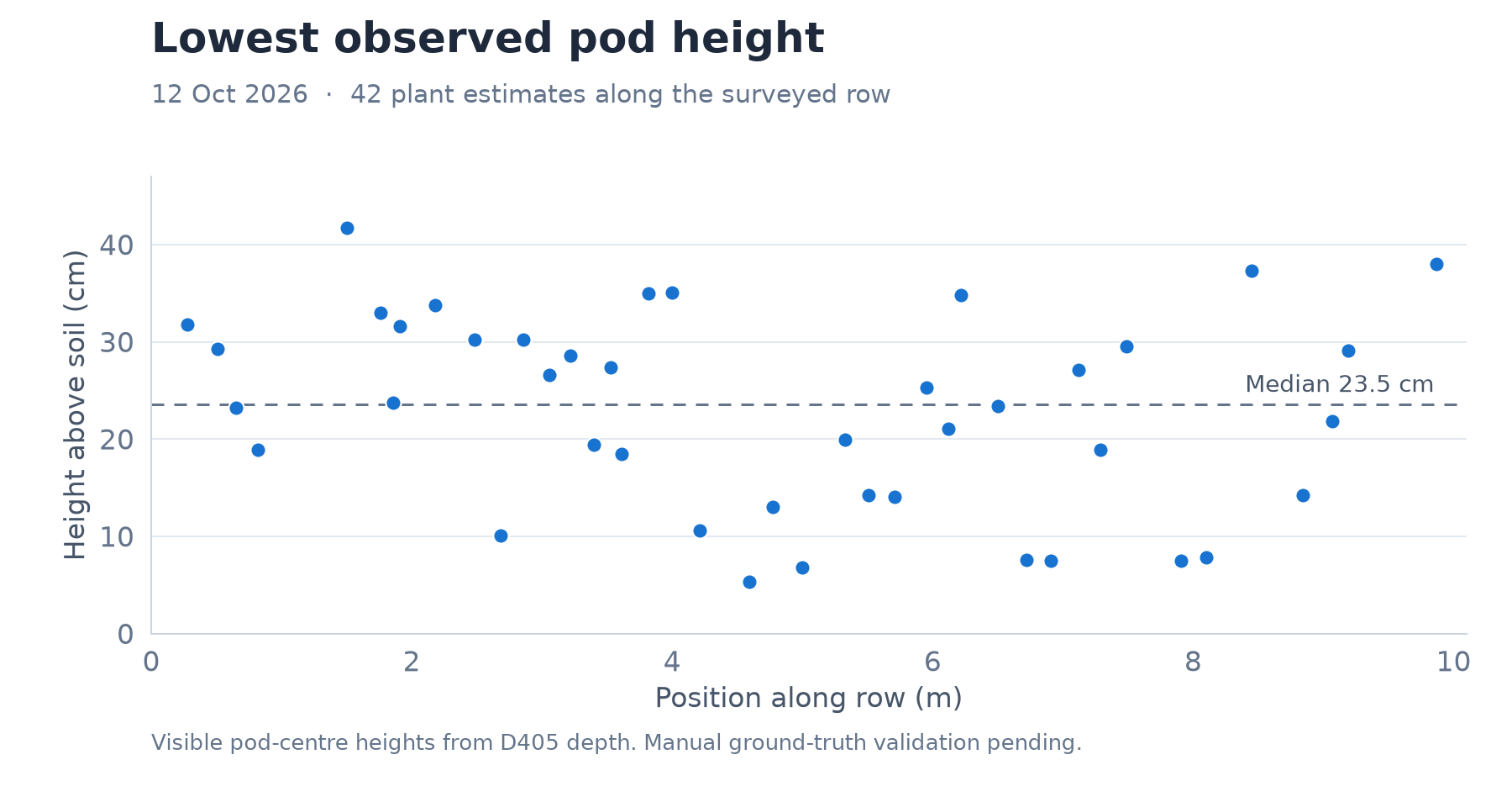
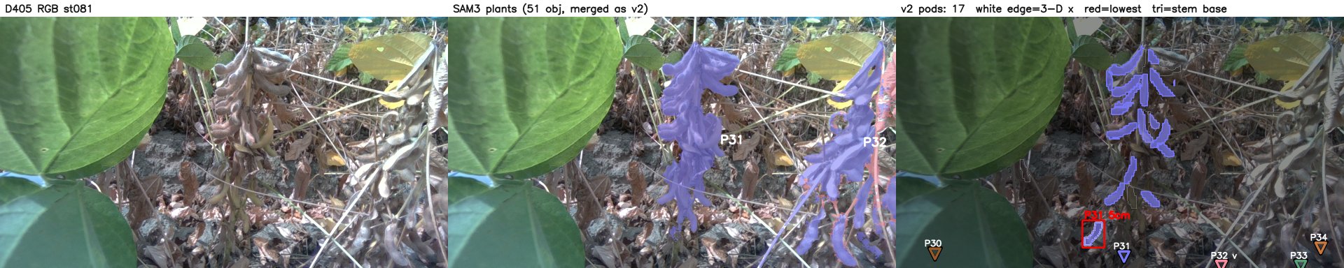
The 12 October r03 survey covered about 9.4 m of mature soybean row. SAM3 plant tracking and PodNet pod detection were combined with measured D405 depth and registered camera poses to reconstruct visible plants and pods. Unlike the earlier presentation's DA3 examples, this result uses the depth sensor directly.
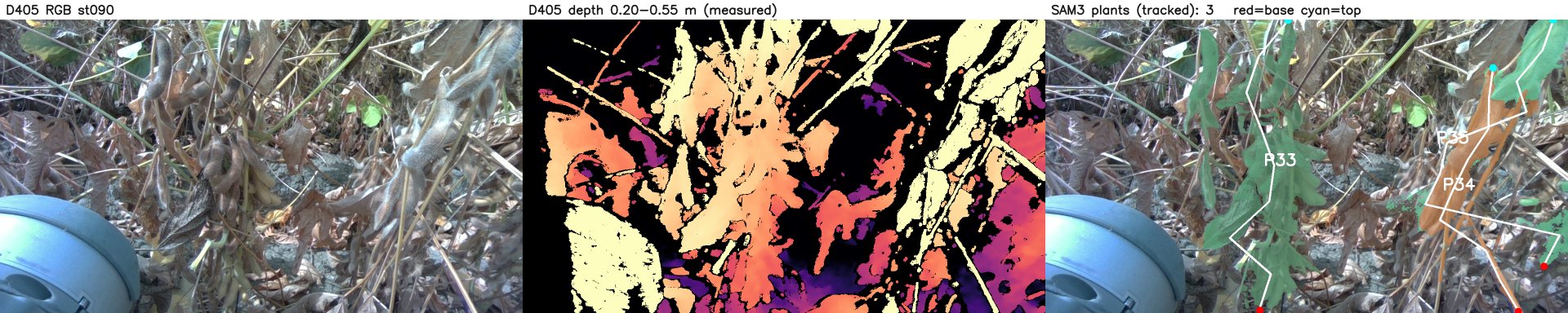
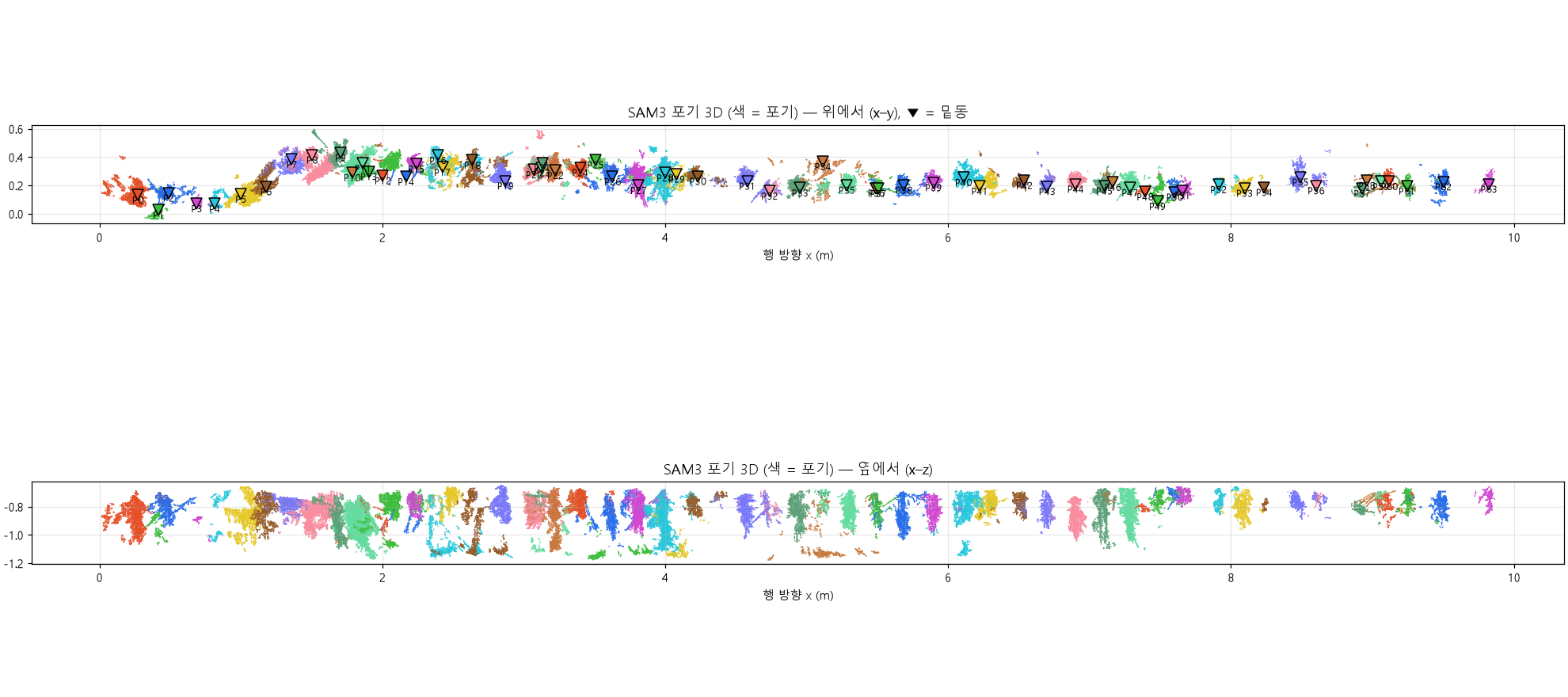
Low stems were used to correct plant bases and merge split tracks. Visible pods outside the plant masks were assigned to nearby bases in 3D. This increased the assigned share of valid pods from 80% to 95%.
| Measure | Result |
|---|---|
| Candidate plants after correction | 55 |
| Plants with pod-height estimates | 42 |
| Valid pods assigned to plants | 392 / 411 (95%) |
| Median lowest observed pod-centre height | 23.5 cm |
| Range across the 42 plants | 5.3–41.7 cm |
Funding
Laboratory research project
This work was supported by the National Research Foundation of Korea (NRF) grant funded by the Korea government (MSIT) (RS-2026-25475333).
Project title: Development of an Integrated Sensing, Monitoring, and Decision-Making Model for Field Surveys in Agricultural Environments (Open Farmland and Greenhouses) Using a Quadruped Robot
Individual research grant
National Research Foundation of Korea (NRF), funded by the Ministry of Education (MOE). Grant RS-2025-25438074.
Project title: Development of Locomotion Algorithms and Autonomous Control Systems for Quadruped Robots Specialized for Korean Agricultural Terrain